
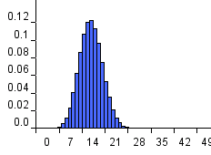
n=10
n=50
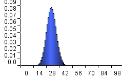
n=100
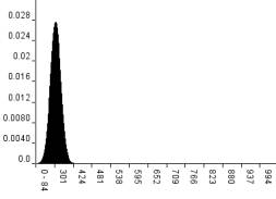
n=1000
You will all have seen or heard statements like the following from pollsters during an election campaign:
Support for candidate Joe Bloggs now stands at 43%. The margin of error is plus or minus three percent.
But what exactly does the statement mean? Most people assume it means that the real level of support for Joe Bloggs must lie somewhere between 40 and 46% with 43% being ‘most probable’. But this is wrong, because there is always an unstated ‘level’ of confidence about the margin of error. Typically, the level is assumed to be 95% or 99%. If pushed, a statistician would therefore expand the above statement as something like:
Statement A: Support for candidate Joe Bloggs now stands at 43%. The margin of error is plus or minus three percent, with confidence at the 95% level.
This combination of the margin of error and the level of confidence about it is what statisticians mean by a confidence interval. Unfortunately, even this more complete statement about the confidence interval is highly misleading. That is because most people incorrectly interpret the statement as being about probability, i.e. they mistakenly assume it means something like:
Statement B: There is a 95% probability that support for candidate Joe Bloggs lies between 40 and 46%.
Statement B is a statement about the probability of the unknown population mean P. Most problems of statistical inference boil down to trying to find out such ‘unknowns’ given observed data. However, there is a fundamental difference between the frequentist approach and the Bayesian approach to probability that was discussed here. Whereas a statement about the probability of an unknown value is natural for Bayesians, it is simply not allowed (because it has no meaning) in the frequentist approach. Instead, the frequentists use the confidence interval approach of statement A, which is not a statement of probability in the sense of Statement B.
It turns out that confidence intervals, as in Statement A, are really rather complex to define and understand properly – if you look at standard statistical textbooks on the subject you will see what I mean. So I will now attempt a proper explanation that is as un-technical as possible.
Being a standard tool of frequentist statisticians the confidence interval actually involves the idea of a repeated experiment, like selecting balls repeatedly from an urn. Suppose, for example, that an urn contains 100,000 balls each of which is either blue or white. We want to find out the percentage (P) of white balls in the urn from a sample of size 100. The previous polling example is essentially the same – the equivalent of the ‘urn’ is the set of all voters and the equivalent of a ‘white ball’ is a voter who votes for Joe Bloggs. The frequentist approach to this problem is to imagine that we could repeat the sampling many times (that is, to determine what happens ‘in the long run’), each time counting the percentage of white balls and adding plus or minus 3 to create an interval. So imagine a long sequence of sample intervals:
[39-45], [41-46], [43-48], [44-49], [42-47], [41-46], [43-48], [39-45], [38-44], [44-49], …
The 95% confidence interval actually means that ‘in the long run’ 95% of these intervals contain the population proportion P.
Now while that is the technically correct definition of a confidence interval it does not shed any light on how statisticians actually calculate confidence intervals. After all, the whole point about taking a sample is
And this is where things get weird. It turns out that, in order to turn your sample proportion into a confidence interval about the (unknown) population proportion P statisticians have to make certain kinds of assumptions about both the nature of the population and the value of the unknown P. This is weird because frequentists feel uncomfortable about the Bayesian approach precisely because of having to make similar kinds of ‘prior’ assumptions.
Of course both the size of the sample and the true value of P will heavily influence the confidence interval. As two extreme cases consider the following:
Example 1: The sample size is 100,000 – i.e. we sample every single ball. In this case the sample proportion p must be exactly equal to the population proportion P. Hence we can conclude that the proportion is exactly P (meaning P plus or minus 0) with confidence at the 100% level (since every time we repeat the procedure we will get this result).
Example 2: The sample size is 1.
In this case the sample proportion must be either 0 (when the sampled
ball is
blue) or 100 (when the sampled ball is white).
So a sequence of samples intervals (based on the plus or
minus 3,
ignoring numbers above 100 and
below 0)
will look like:
Unless P is either between 0 and 3 or between 97 and 100 there is no non-zero confidence interval that will work. However, if we use plus or minus 50 for our intervals then we would get:
[0-50], [0-50], [50-100], [0-50], [50-100], [50-100], [50-100], [0-50], [50-100], …
Suppose that 80% of these intervals are of the type [0-50]. Then we would be able to conclude the following:
The proportion of white balls is 0%. The margin of error is plus or minus 50%, with confidence at the 80% level.
Or,
equivalently
The proportion of white
balls is 25%. The margin of error is plus or minus 25%, with confidence
at the
80% level.
Neither of these statements is
especially useful, which suggest that unless we already have a good
idea about
what P is, we will need a reasonable size sample to conclude anything
helpful.
Both examples highlight a real dilemma regarding the use of confidence intervals. Although the formal definition assumes some notion of a ‘long run’ of similar samples, such long runs are not intended to take place (that would otherwise defeat the whole objective of doing sampling). So what the frequentists have to do is come up with some analytical methods for predicting what might happen in the long run. In the case of example 1 this is easy. Analytically we know that every sample of size 100,000 is guaranteed to produce a proportion p that is exactly equal to the population proportion P. But what can we say if the sample is, say 1,000? Suppose that, in that sample, we find that p=30%. How do we turn this into a confidence interval?
This is where statisticians have to make certain kinds of assumptions about both the nature of the population and the value of the unknown P.
As is shown in the section on maxium likelihood estimation, with certain assumptions about the population and the sampling strategy, it turns out that the most likely value of the population proportion P is actually equal to the sample proportion p. So if we assume that the population proportion is indeed equal to p, then for a sample of size n we can calculate the probability that the sample proportion will be within some interval of p (for example p plus or minus 0.01*p). Suppose that our sample size is 10 and that in our sample we found 3 white balls. Then, assuming the population proportion is the same as the sample proportion 0.3 we can ask: for any sample of size 10 what is the probability that the sample proportion is between 0.2 and 0.4? This turns out to be a classic case of the Binomial distribution. The top left graph of the FIGURE below shows the Binomial distribution needed. Because n is quite small the variance of the distribution is quite large. It turns out that the probability the sample proportion will lie between 0.2 and 0.4 is about 0.74. So in the long run we expect that 74% of all samples of size 10 will have a sample proportion of between 0.2 and 0.4. Hence, if we observe 3 white balls from a sample of size 10, we can conclude the following:
The proportion of white balls in the urn is 30% plus or minus 10%, with confidence at the 74% level.
However, as we increase the sample size (see the FIGURE) note how the Binomial distribution variance decreases, i.e. the distribution becomes much more sharply focused around the mean. The effect of this is that if we found 300 white balls when the sample size n=1000 then we can conclude the following:
The proportion of white balls in the urn is between 29% and 31%, with confidence at the 95% level.
So, as the sample size n increases we can make stronger statements in the sense that the interval around the sample mean decreases while the confidence level increases.
|
n=10 |
n=50 |
|
n=100 |
n=1000 |
Figure 1 Binomial distribution for different values of n when p=0.3
In practice the Binomial distribution is rather awkward to use to calculate confidence intervals. As shown in <NORMAL> the bell curve, or Normal distribution, is a good approximation of the Binomial in the case where n is large and p is not close to 0 or 1 (indeed FIGURE above shows how the Binomial becomes increasingly like the Normal as n increases).
The key thing about a Normal distribution is that 95% of the distribution lies between the mean of the distribution plus or minus 1.96 times the standard deviation as shown in FIGURE.
Figure 2 The Normal distribution and its 95% confidence interval
So, once we know the mean and the standard deviation s we can calculate the 95% confidence interval using the formula:

Now the Binomial distributions above all have mean equal to n*p (where n is the sample size and p is the proportion of white balls) and standard deviation s is equal to
Thus, for example, when n =10 and p=0.3, the mean is equal to 3 and the standard deviation is approximately equal to 1.45. Other values are shown in the table.
|
n |
p |
mean |
Standard deviation |
95% CI |
95% CI as percentage |
|
10 |
0.3 |
3 |
1.45 |
3±2.84 |
30±28.4 |
|
50 |
0.3 |
15 |
3.24 |
15±6.35 |
30±12.7 |
|
100 |
0.3 |
30 |
4.58 |
30±8.98 |
30±8.98 |
|
200 |
0.3 |
60 |
6.48 |
60±12.7 |
30±6.35 |
|
1000 |
0.3 |
300 |
14.49 |
300±28.4 |
30±2.84 |
|
5000 |
0.3 |
1500 |
32.4 |
1500±63.51 |
30±1.27 |
The 95% confidence interval is then 3±2.84.
Other values for confidence intervals as we increase the sample size (while still observing 30% white balls in the sample) are shown in the table. Thus, for example, if we observed 1500 white balls in a sample of size 5000, then the mean of the distribution is 1500±63.51 at the 95% confidence interval.
Normally instead of a confidence interval about the population mean we prefer to speak in terms of a confidence interval about the population percentage (i.e. in this case the percentage of white balls) as shown in column 6 of the table. To turn a confidence interval about the mean into a percentage you simply multiply by 100/n where n is the sample size.
As is clear from the table the 95% confidence intervals gets increasingly close to 30% as the size n of the sample increases.
In general there is no reason to restrict ourselves to 95% confidence intervals. Exactly the same technique can be applied, for example, to 90% (where we use a multiplier of 1.64 instead of 1.96) or 99% confidence intervals (where we use a multiplier of 2.58). More generally there are tables for the Normal distribution that can be used for arbitrary values of the confidence interval.
As we said at the beginning, the use of confidence intervals is the standard frequentist approach to reasoning about an unknown population mean. The Bayesian approach is conceptually simpler. See here to find out how Bayesians handle the problem.