[papers/_private/small_logo.html]

New Directions The results in Section 4 provide mixed evidence about the usefulness of the commonly used metrics. Results for hypotheses 1, 2,3, 7 and 8 explain why there is still so much interest in the potential of defects data to help quality prediction. But the other results confirm that the simplistic approaches are inevitably inadequate. It is fair to conclude that complexity and/or size measures alone cannot provide accurate predictions of software defects on its own, information about software defects (discovered pre-release) provides no information about likely defects post-release. traditional statistical (regression-based) methods are inappropriate for defects prediction In addition to the problem of using metrics data in isolation, the major weakness of the simplistic approaches to defect prediction has been a misunderstanding of the notion of cause and effect. A correlation between two metric values (such as a module’s size and the number of defects found in it) does not provide evidence of a causal relationship. Consider, for example, our own result for hypothesis 4. The data we observed can be explained by the fact that the modules in which few faults are discovered during testing may simply not have been tested properly. Those modules which reveal large numbers of faults during testing may genuinely be very well tested in the sense that all the faults really are 'tested out of them'. The key missing explanatory data in this case is, of course, testing effort, which was unfortunately not available to us in this case study. As another example, hypothesis 5 is the popular software engineering assumption that small modules are likely to be (proportionally) less failure prone. In other words small modules have a lower defect density. In fact, empirical studies summarised in [Hatton 1997] suggest the opposite effect: that large modules have a lower fault density than small ones. We found no evidence to support either hypothesis. Again this is because the association between size and fault density is not a causal one. It is for this kind of reason that we recommend more complete models that enable us to augment the empirical observations with other explanatory factors, most notably, testing effort and operational usage . If you do not test or use a module you will not observe faults or failures associated with it. Thus, the challenge for us is to produce models of the software development and testing process which take account of the crucial concepts missing from traditional statistical approaches. Specifically we need models that can handle: diverse process and product evidence genuine cause and effect relationships uncertainty incomplete information At the same time the models must not introduce any additional metrics overheads, either in terms of the amount of data-collection or the sophistication of the metrics. After extensive investigations during the DATUM project 1993-1996 into the range of suitable formalisms [Fenton et al 1998] we concluded that Bayesian belief nets (BBNs) were by far the best solution for our problem. The only remotely relevant approach we found in the software engineering literature was the process simulation method of [Abdel-Hamid 1991], but this did not attempt to model the crucial notion of uncertainty. BBNs have attracted much recent attention as a solution for problems of decision support under uncertainty. Although the underlying theory (Bayesian probability) has been around for a long time, building and executing realistic models has only been made possible because of recent algorithms (see [Jensen 1996]) and software tools that implement them [Hugin A/S]. To date BBNs have proven useful in practical applications such as medical diagnosis and diagnosis of mechanical failures. Their most celebrated recent use has been by Microsoft where BBNs underlie the help wizards in Microsoft Office. A number of recent projects in Europe, most of which we have been involved in, have pioneered the use of BBNs in the area of software assessment (especially for critical systems) [Fenton et al 1998], but other related applications include their use in time-critical decision making for the propulsion systems on the Space Shuttle [Horvitz and Barry 1995]. 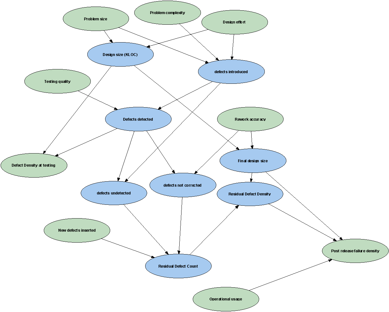A BBN is a graphical network (such as that shown in Figure 2) together with an associated set of probability tables. The nodes represent uncertain variables and the arcs represent the causal/relevance relationships between the variables. The probability tables for each node provide the probabilities of each state of the variable for that node. For nodes without parents these are just the marginal probabilities while for nodes with parents these are conditional probabilities for each combination of parent state values. The BBN in Figure 2 is a simplified version of the one that was built in collaboration with the partner in the case study described in Section 4. Figure 2: A BBN that models the software defects insertion and detection process It is simplified in the sense that it only models one pre-release testing/rework phase whereas in the full version there are three. Like all BBNs the probability tables were provided by a mixture of: empirical/benchmarking data and subjective judgements. We have also developed (in collaboration with Hugin A/S) tools for generating quickly very large probability tables. It is beyond the scope of this paper to describe either BBNs or the particular example in detail (see [Fenton and Neil 1998] for a fuller account). However, we can give a feel for its power and relevance. First note that the model in Figure 2 contains a mixture of variables we might have evidence about and variables we are interested in predicting. At different times during development and testing different information will be available, although some variables such as ‘number of defects inserted’ will never be known with certainty. With BBNs, it is possible to propagate consistently the impact of evidence on the probabilities of uncertain outcomes. For example, suppose we have evidence about the number of defects discovered in testing. When we enter this evidence all the probabilities in the entire net are updated. 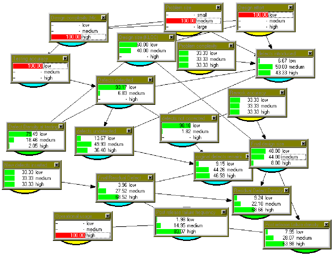In Figure 3 we provide a screen dump from the Hugin tool of what happens when we enter some evidence into the BBN. In order for this to be displayed in one screen we have used a massive simplification for the range of values in each node (we have restricted it to 3 values: low, medium, high), but this is still sufficient to illustrate the key points. Where actual evidence is entered this is represented by the dark coloured bars. For example, we have entered evidence that the design complexity for the module is high and the testing accuracy is low. When we execute the BBN all other probabilities are propagated. Some nodes (such as ‘problem complexity’) remain unchanged in its original uniform state (representing the fact that we have no information about this node), but others are changed significantly. In this particular scenario we have an explanation for the apparently paradoxical results on pre-and post-release defect density. Note that the defect density discovered in testing (pre-release) is likely to be ‘low’ (with probability 0.75). However, the post-release failure density is likely to be ‘high’ (probability 0.63). Figure 2: Entering evidence into the BBN — an explanation for the ‘paradox’ of low defect density pre-release but high defect density post-release This is explained primarily by the evidence of high operational usage, low testing accuracy, and to a lesser extent the low design effort. The example BBN is based only on metrics data that was either already being collected or could easily be provided by project personnel. Specifically it assumes that the following data may be available for each module: defect counts at different testing and operation phases size and ‘complexity’ metrics at each development phase (notably LOC, cyclomatic complexity) the kind of benchmarking data described in hypotheses 7 and 8 of Table 1 approximate development and testing effort At any point in time there will always be some missing data. The beauty of a BBN is that it will compute the probability of every state of every variable irrespective of the amount of evidence. Lack of substantial hard evidence will be reflected in greater uncertainty in the values. In addition to the result that high defect density pre-release may imply low defect density post-release, we have used this BBN to explain other empirical results that were discussed in Section 4, such as the scenario whereby larger modules have lower defect densities . The benefits of using BBNs include: explicit modelling of ‘ignorance’ and uncertainty in estimates, as well as cause-effect relationships makes explicit those assumptions that were previously hidden - hence adds visibility and auditability to the decision making process intuitive graphical format makes it easier to understand chains of complex and seemingly contradictory reasoning ability to forecast with missing data. use of ‘what-if?’ analysis and forecasting of effects of process changes; use of subjectively or objectively derived probability distributions; rigorous, mathematical semantics for the model no need to do any of the complex Bayesian calculations, since tools like Hugin do this Clearly the ability to use BBNs to predict defects will depend largely on the stability and maturity of the development processes. Organisations that do not collect the basic metrics data, do not follow defined life-cycles or do not perform any forms of systematic testing will not be able to apply such models effectively. This does not mean to say that less mature organisations cannot build reliable software, rather it implies that they cannot do so predictably and controllably.   To go back to our resources section click here.

[papers/_private/horizontal_navbar.html]

[papers/_private/copyright_notice.html]

Last modified: July 28, 1999.