Software Metrics Programs:setting up a useful program may be easier than you thinkQuick Summary You do not need fancy metrics and models for a useful metrics program. This is especially true if you want metrics to help with quality control and assurance. What you need most is good data about defects. Contents
Your starting point: distinguishing between faults and failures If your organisation makes a conscious effort to record information about its software defects then you may be pleasantly surprised to know that you already have in place the basics of a metrics program. However, it is also likely that you are either not making much use of the information, or even worse, getting misleading results out of it. Typically, you might see the kind of data shown in the first two or four columns of Table 1 (this is based on a real sample of modules from a major system). Table 1: Typical summary defects data (high outliers in each column are highlighted)
In this case the development organisation was quite rigorous in its approach to recording defects. Every defect discovered during independent testing and in operation was traced to a specific software module. The organisation wanted to identify ‘problem’ modules out of the hundreds in total. The raw defects data (columns 1 and 2) suggests that modules Q and L are the problem modules. In many cases this is as far as your data will allow you to go. Yet, looking a bit deeper reveals a very different story. First, recovering the module size data in thousands of lines of code (KLOC) and taking it into account (columns 3 and 4) immediately ‘explains’ the problem with module Q. It's big. We might now conclude that A and L are the problem modules because they have the most defects per line of code. However, when the defects are split between those that were discovered by testers pre-release (column 5) and those that were the cause of customer-reported problems post-release, then the picture is completely different. The ‘problem’ modules post-release are C and P. Sidebar: Definitions relevant for software ‘defects’ Software failure: a deviation from expected or required behaviour of the software in operation Software fault is the encoding of a human error into the software; in this context we include documentation, such as the specification or user manual, as software and we include ‘omissions’ as faults. Software defect is the collective term used for fault or failure Pre-release fault: a fault discovered (internally) before software is releases to customer Post-release fault: the cause of an observed failure The problem with the basic data is that a ‘defect’ is referring to two very different concepts� faults and failures. The definitions for these, and related, terms is given in Sidebar 1. Although every failure is caused by some fault(s), a fault will only trigger a failure under certain inputs and operating conditions. The post-release faults are those that have actually caused operational failures (unlike the pre-release faults which may or may not cause such failures if they were not fixed). For simplicity, let us assume that there is roughly a one-to-one correspondence between failures and post-release faults (in reality some failures are caused by more than one fault and some faults cause different failures, but in practice the total numbers turn out to be roughly equal). Now, most people who collect fault data pre-release are really interested in using it to predict the number of post-release failures. With our assumptions, Table 1 highlights just how bad the pre-release fault data is at predicting post-release failures at the module level. Generally, there is now very good empirical evidence that pre-release faults is a bad predictor of post-release faults. Figure 1 shows the results of a recent study of a major telecommunication software system. The modules with most faults pre-release generally had very few post-release. Conversely, the genuinely failure-prone modules generally have low numbers of pre-release faults. For this system some 80% of pre-release faults occurred in modules which had NO post-release faults. Similar results have been observed for other systems.
Figure 1: Relationship between modules' pre- and post-release fault counts (each dot represents a randomly selected module) A high number of pre-release faults may simply be explained by good testing rather than poor quality. A low number of post-release faults may simple be explained by low operational usage. In fact, the relationship between faults and failures is not at all straightforward. There is very strong empirical evidence that most failures experienced by software systems are caused by a very tiny proportion of the residual faults. Conversely, most residual faults are benign in the sense that they will very rarely lead to failures in operation. This is shown in Figure 2.
Figure 2: The relationship between faults and failures In 1983 Ed Adams of IBM published the results of an extended empirical study into the relationship between faults and failures in nine large systems over many years of operation. He found remarkably consistent results between the nine systems. For example, in each case around 34% of the known residual faults led to failures whose mean time to occurrence was over 5,000 years. In practical terms such failures were probably only ever observed once by a single user (out of many thousands of users over several years). Conversely, the ‘big’ faults� those which cause the frequent failures (with mean time to occurrence of less than 5 years)� made up less than 2% of the faults. The consequences of the Adams’ phenomenon are quite serious for metrics based simply on fault counts. In Table 1 the pre-and post-release faults were lumped together in column 2 and a derived metric 4, defect density (defects/KLOC), was calculated. Many companies use this metric as a de-facto quality measure. Even ignoring the problems with using KLOC as a size measure, this metric is almost meaningless when ‘defects’ effectively lumps together faults and failures. It makes more sense to compute the fault density metric separately for pre-and post-release faults. Providing that possible explanatory factors are taken into account, the pre-release fault density metric has some merit as a purely internal pre-release quality control mechanism. The metric can be especially useful when used in outlier analysis: very low values may be indicative of good design or may simply indicate that insufficient testing was done. Either way it is extremely useful to know which modules really are outliers (either low or high) as this is the first place to look for process improvement. The post-release fault density metric has some merit as a quality measure, providing that the failures are recorded during some well-specified operational conditions (such as first 100 hours of operation by an experienced user). What should be clear so far is the importance of distinguishing between faults and failures (and hence between pre- and post-release faults) in any data-collection program. It is also clear that, if we want to use fault data for useful prediction, we need to get some additional information. It is that information which defines a metrics program. Identifying your metrics goalsA metrics program is any planned activity of using measurement to meet some specific goal. If you do not have a clear technical goal for a metrics program, then you are almost certainly not ready for such a program. If, for example, your only reason for instigating a metrics program is to satisfy some external assessment body or achieve a higher level on some process maturity scale, then your metrics program is a ‘grudge purchase’. It will almost certainly fail because of lack of focus and motivation.
Figure 3: The necessary chain for a successful metrics activity Even if you have a specific technical goal the program is doomed to fail unless it leads (as shown in Figure 3) to decisions and a potential set of actions. For example, if your goal is to assess the effectiveness of two different testing tools being used by members of staff, then the measurement results might lead you to decide that one tool is more effective overall than the other. In that case the decision should result in the action not to continue with the less effective tool. If such an action was always beyond your control then the measurement program was a waste of time; the next time you try to set one up your staff will be less likely to co-operate. Because there are many different technical goals that can be supported by metrics, there is no such thing as a metrics program to suit all. I do not therefore believe in the notion of an all-embracing ‘company-wide’ metrics program. It is impossible to define a uniform set of metrics. Everything depends on what your goal is for measurement. The first section described metrics commonly used by companies that deliver large systems in phased releases. The metrics revolve around the testing process. Suppose such a company A's goal is to monitor ‘quality’ over time and identify those components of the systems that are especially failure-prone. We'll use that goal in the remainder of the paper. But there are other possible goals. Suppose Company B’s goal is to improve the way they estimate project resources at the requirements phases of new projects. They need completely different metrics that characterise properties of their project requirements and metrics that relate to project resources. They will need to collect such metrics for a number of similar projects before they can predict, with confidence, the likely resources for a given set of requirements. Having identified the technical goal, it is helpful next to formulate some questions that help clarify your goal in measurable terms. This is shown in Figure 4 for Company A’s example. The questions in turn give rise to a number of metrics that might help you answer them. This is the so-called Goal-Question-Metric (GQM) approach.
Figure 4: Goal-Question-Metric approach
Having applied an approach like GQM you will have some idea of what metrics you would ideally like and why they can address your goal. In practice it will be impossible to get all the metrics that arise from a high-level GQM strategy. For example, we know that the ‘size’ (in terms of functionality) and ‘complexity’ (in terms of difficulty) of a module are certain to be key factors in the number of faults you will find. However, it may be impossible to get accurate measures of functionality and complexity; you may have to be satisfied with simple counts like KLOC and number of code branches. Similarly, we know that the amount of operational usage of a module is a key factor in the number of failures it is reported to cause; however, you may have no way of finding out such data. It is your task, therefore, to formulate a realistic metrics plan, which effectively acts as the specification for your ‘metrics program’. This document should contain the basic information shown in Table 2.
Table 2: Basic components of the metrics plan
For company A, this might be something like:
A rigorous defects database and its use in the metrics program For a measurement goal like Company A’s it should be clear by now that much of the necessary metrics information should already be routinely collected as part of a configuration management and defect reporting system. We are not proposing a new dedicated metrics database. We have found from inspecting various company systems that simple changes to the existing defects database can often increase drastically the potential for metrics to be used effectively. For example, many companies make the mistake of treating faults and failures equally in their defect reporting system. This approach runs into the major problems already highlighted. Such an approach also leads to very poor information in the database� this is almost inevitable if people are expected to complete exactly the same kind of information about failures as faults. Our preferred approach is to think of the database as containing information about issues. An issue is a failure, fault, or a change request. Users report failures when the system is operational. Faults are either found by testers pre-release, or they are the result of finding the cause of a failure. Change requests (for new functionality) may be reported by users or developers. Failures have attributes like: Faults also have attributes location and timing but location refers to the relevant configuration item (such as a particular module) and timing refers to the testing phase (module testing, system testing, integration testing, post-release). All issues should have a criticality and/or severity attribute (criticality refers to the importance of the issue whereas severity refers more to its size; for example the criticality of a failure could be classified as major if it causes a complete system crash, while its severity could be classified as major if it is likely to affect a lot of users). It is not difficult to build a relational database in such a way that we can relate:
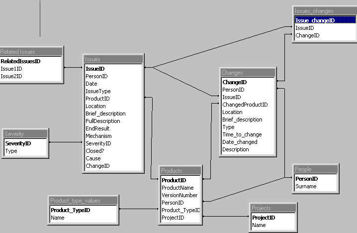
An example of the relational structure is shown in Figure 5
Figure 5: Relational structure for database We have built an effective database using three basic forms:
Figure 6: Example Issues Form To make this data-collection process work well and to integrate fully into the metrics program, it is necessary to have the commitment of the project manager. Specifically, this must be the place where all issues are reported and channeled. Not just metrics programs but also general fault-reporting and configuration management procedures can be fatally compromised if there is some alternative covert channel for raising and resolving issues. Also, one key person (probably the project manager) should be responsible for filtering entries to ensure that only genuinely new issues are entered into the database. Otherwise, not only is there multiple counting of the same failures and faults, but time is wasted repeating work. It is instructive to see how the database can help us follow through the chain of activities shown in Figure 3. Based on the example of Company A, we have already seen how GQM and the metrics plan addresses the goals and metrics. The database will certainly enable us to extract the kind of data shown in Table 1. However, unlike the position we started from, we will be able to get the full information, including the crucial last three columns. This data allows us to observe facts/trends like:
However, we have already identified in our metrics plan possible explanatory/predictive factors. We can extract these factors from the database. For example, by simply applying a filter we could restrict our defect density analysis to only the most serious/critical defects to see if this changes the picture. For modules with very low pre-release defect density we could check their testing effort and compare it with the lowest/average/highest for all modules. We might find, for example, that all of the modules B,C,and I that recorded zero pre-release faults had a significantly below average testing effort. Information such as this may lead to decisions such as that certain modules really do need extra testing or completely redesigning before release. These decisions should lead to the associated actions and more general actions such as putting in place new QA procedures (such as minimum levels of testing).
Future DirectionsThe need to take account of explanatory and causal factors is paramount if you wish to use metrics as a real management tool for risk reduction. For example, fault density values become irrelevant if you know that certain modules have not been tested at all. Simply knowing that certain modules are problem modules is a useful first step, but does not help you to know how to intervene to avoid such problems in the future. The key to more powerful use of software metrics is not in more powerful metrics. Rather it is in a more intelligent approach to combining different metrics. We have provided some general guidelines about how to do this. Once you are comfortable with such an approach you may need to look at more advanced statistical techniques for achieving a real prediction system. Bayesian Belief nets (BBNs) is such an approach that we feel provides the most promising way forward. We have been using BBNs to improve predictions of software quality by taking account of causal factors, and we have also used BBNs to define appropriate risk-reduction intervention strategies. |